Volt argues that a vanilla transformer, with the right recipe and enough data, no longer needs a convolution-specialized backbone for 3D scene understanding. We took that seriously, reproduced it in WarpConvNet, and asked a narrower question. In the regime the paper itself flags as hard (single dataset, from scratch, no teacher), does putting the convolutional inductive bias back into the architecture help? It does. A sparse-conv stem and a per-block conv reach 78.23 mIoU on ScanNet from scratch, and the effect grows with model size: at the width we deploy, the conv stem alone is worth +1.70 mIoU, while scaling the transformer without it buys only +0.47.
What Volt claims
Volt (Volume Transformer, ECCV 2026) makes a clean argument. 3D scene understanding has been stuck on specialized backbones with strong domain priors, and that isolation costs the field the momentum of the broader transformer stack. So Volt adapts a vanilla transformer to 3D with minimal changes: partition the scene into volumetric patch tokens, run full global self-attention, and inject position with a 3D rotary embedding. It shows the result can be competitive with, and at scale beat, the conv-specialized incumbents.
It’s a good argument, and the paper is careful about where it holds. Two of its own points matter here:
“Naively training Volt on standard 3D benchmarks leads to shortcut learning, highlighting the limited scale of current 3D supervision.”
That is the paper conceding the small-data regime is hard for a pure transformer. Its remedy is a data-efficient recipe (strong 3D augmentation, regularization, and distillation from a convolutional teacher), plus joint training across multiple datasets for the headline results. The “you don’t need conv backbones” conclusion is really a statement about scale: given enough supervision, global attention wins.
Notice what the small-scale recipe does, though. It reaches for a convolutional teacher. The conv inductive bias doesn’t disappear; it gets imported through distillation rather than built into the model. That is the thread we pulled.
The question we asked
We deliberately stayed in the corner the paper flags as hard: a single dataset (ScanNet v2), trained from scratch, with no distillation teacher. This is the setting most practitioners live in, with one labeled dataset and no pretrained conv oracle on hand.
The question: if the conv inductive bias is worth importing via a teacher at this scale, is it worth building directly into the architecture, and how much does it buy?
Reproduce first
Before touching anything, we confirmed the baseline was reachable. The from-scratch Volt-S
config reproduced 76.26 mIoU (TTA) against the paper’s reported 77.3. We then reimplemented
Volt natively in WarpConvNet (tokenizer, anisotropic axial RoPE, RoPE attention over
flash_attn_varlen_qkvpacked, linear detokenizer, all speaking the Voxels type), and it
scored 76.06, within noise of our own 76.26.
Two caveats. Our from-scratch reproduction lands about a point under the paper’s reported 77.3, plausibly down to schedule and recipe differences, so treat the cross-paper number as context rather than a controlled comparison. The reliable signal is internal: every variant below is trained with the identical recipe and schedule, so each delta is attributable to the one thing we changed. Baseline to beat: 76.06.
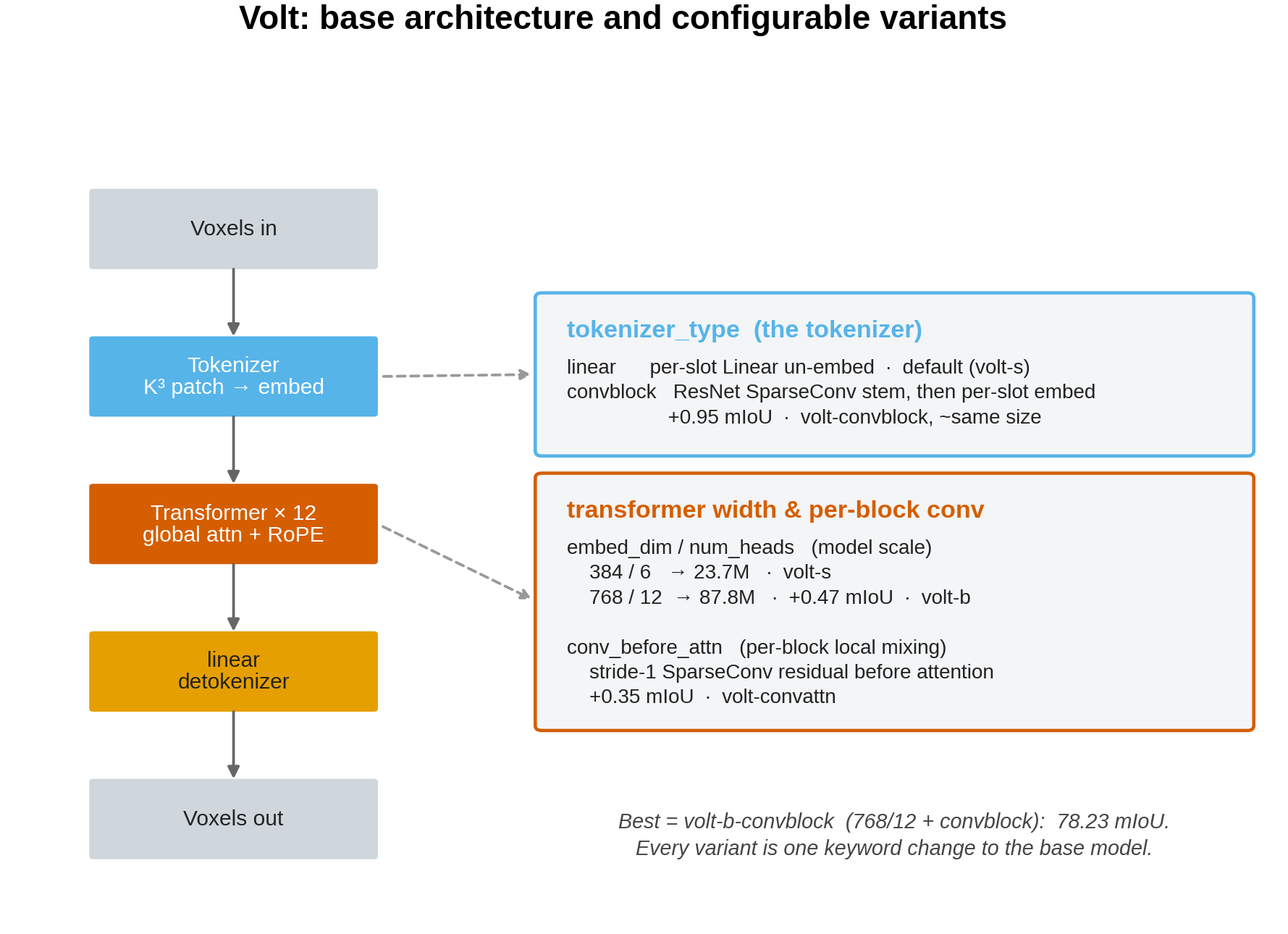
Volt has no convolutions and no hierarchy: global attention at a single coarse scale, and a linear map at each end. That leaves a clean substrate, with exactly two seams where a convolutional bias can be reintroduced without disturbing the global-attention core.
Seam one: the tokenizer
The stock tokenizer scatters the voxels of each 5³ patch into 125 slots, flattens to a
[P, 750] vector, and applies one Linear. It is lossless within a patch and blind across
patch boundaries: a voxel one step outside the patch might as well not exist.
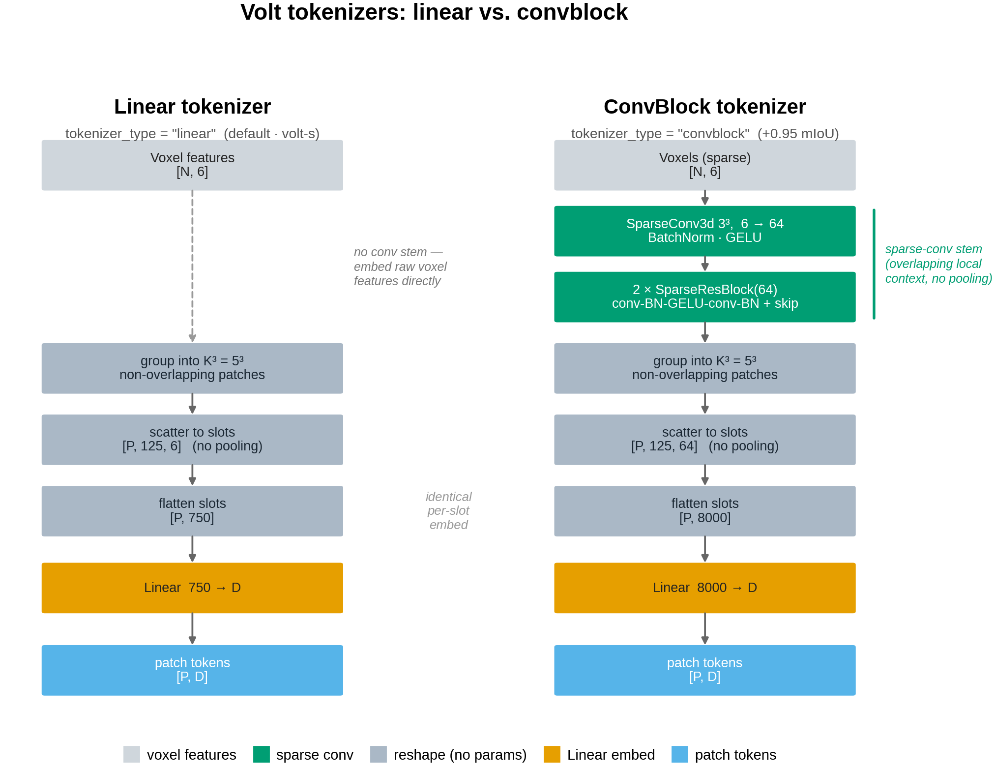
Our first attempt was the naive one, a sparse-conv stem that pools each patch with
scatter_mean. It lost 1.26 mIoU (74.80). Mean-pooling destroys exactly the within-patch
structure the linear embed was preserving. Only one class improved, picture, which is thin
and relies on cross-patch overlap, and that pointed at the fix: add locality alongside the
per-slot embed, not in place of it.
The convblock tokenizer does that. A non-strided sparse-conv stem (SparseConv3d → BN →
GELU, then two residual sparse-conv blocks) gives every voxel overlapping local context, and
then the original scatter → flatten → Linear runs unchanged. Same output size, same
parameter count, no pooling. It gained +0.95 mIoU (77.01), the largest single change we
found, from a stem that costs almost nothing.
Seam two: the transformer block
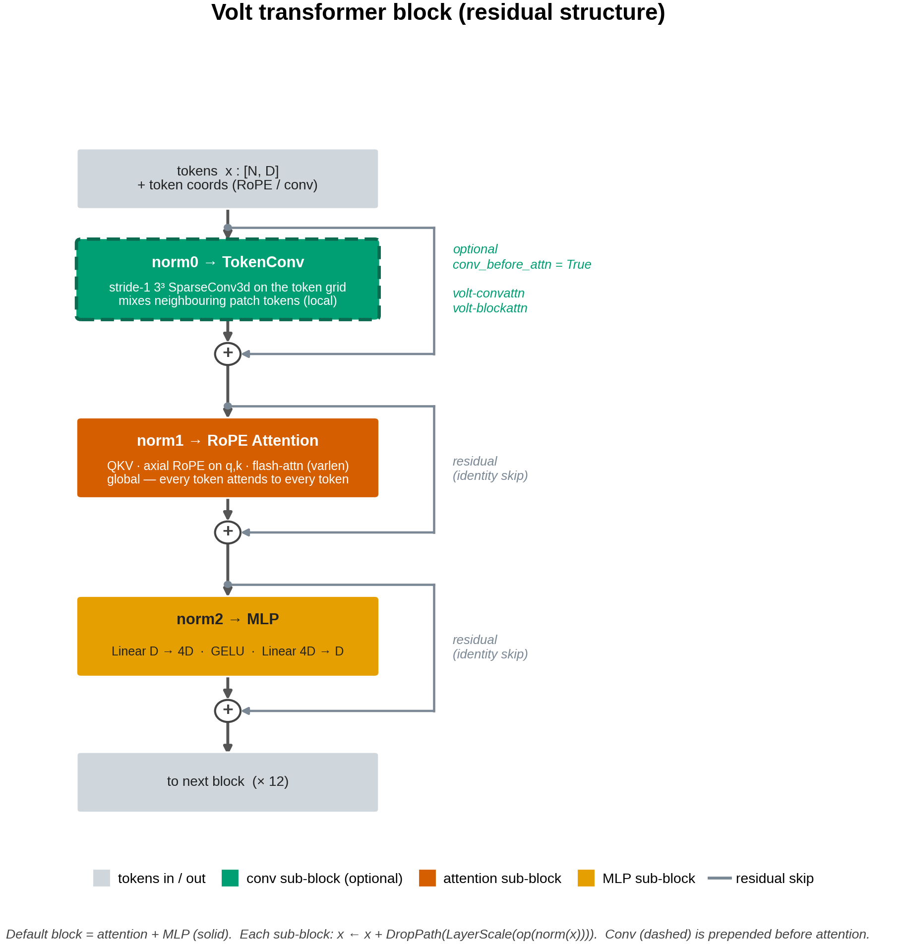
The second seam is inside each of the 12 blocks. conv_before_attn prepends one more
residual sub-block, a stride-1 3³ sparse convolution over the token grid, before attention.
Each layer then mixes neighbouring patch tokens locally first, then attends globally.
On its own it is worth +0.35 mIoU (76.41). Smaller than the stem, but it moves different
classes, the fine and boundary categories like picture, desk, and window, which matters
when we stack.
For reference, plain width (embed_dim 384→768) is +0.47 (76.53) and helps the large,
structured classes, table and bookshelf. Capacity and locality act on different
weaknesses.
Isolating the convolutional bias
To measure what the conv stem contributes, the right baseline is the same-width model without it, not the smallest model. Our best config is Volt-B with the stem, so Volt-B without the stem is the reference. The four configs form a 2×2 over {tokenizer × width}:
| linear tokenizer | + convblock stem | conv effect | |
|---|---|---|---|
| 384-d (Volt-S) | 76.06 | 77.01 | +0.95 |
| 768-d (Volt-B) | 76.53 | 78.23 | +1.70 |
| width effect | +0.47 | +1.22 |
Two things fall out of the table. The conv stem helps at both widths, and more at the larger one: +1.70 at Volt-B versus +0.95 at Volt-S. And scaling the transformer on its own, the lever Volt leans on, buys just +0.47 without the stem against +1.22 with it. Capacity and the convolutional bias reinforce each other. Each is worth more in the presence of the other, and the best cell is the one with both. This holds only because the stem sits alongside the per-slot embed; the mean-pool version, which replaced it, lost 1.26.
The third knob, and where stacking stops
The per-block conv (conv_before_attn, +0.35 at base width) is a second, independent way to
inject locality. Stacked with the conv stem at base width it reaches 78.00
(convblock + conv-before-attn, 74.7M), and the two local-mixing mechanisms compose, with
broad gains across bed, door, picture, and otherfurniture.
Adding it on top of the conv stem and width is where the story turns. All three at once (768-d + convblock + conv-before-attn, 285M) scores 77.93, below either two-way combination. Once the model already has one source of local mixing and the extra width, a second conv injection plus 190M more parameters buys nothing but a little overfit. Conv-stem and width compound; conv-stem and per-block conv are redundant.
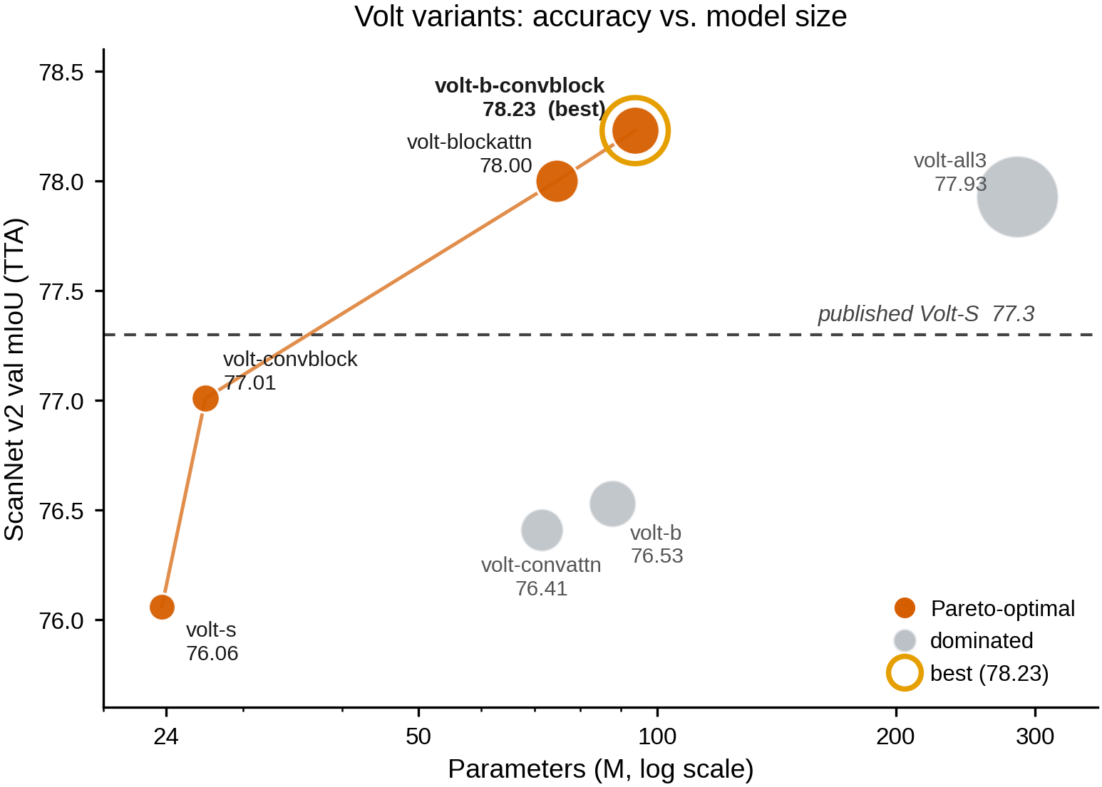
The Pareto view gives the practical read. The convblock stem alone, which is nearly free,
reaches the published number. convblock + width is the accuracy pick. Everything to its
right, including the 285M kitchen sink, is dominated.
Why it works: the bias rescues the weak classes
The per-class breakdown is where the inductive-bias story shows up directly. The convblock
stem lifts the weak, boundary-sensitive classes: door, picture, fridge, wall. These
are precisely the categories the linear tokenizer starves of cross-patch context. Give them
local receptive fields and they recover. Width, on the other hand, lifts the large,
structured classes, table and bookshelf, which want capacity rather than locality.
Because they repair different failure modes, they add. And because conv_before_attn and the
convblock stem both inject locality, once you have one, a wider model does not need the
other, which is why all3 regresses. The gains stack when the two changes do different jobs,
not when you pile on more of the same.
That pattern is the point. At this data scale, global attention alone leaves the small, thin, boundary-heavy classes underserved, and a modest convolutional bias (a few sparse convs, no pooling, no teacher) is what pulls them up.
Reading it back against Volt’s thesis
We are not contesting Volt’s main claim. At multi-dataset scale, with the full recipe, a vanilla transformer may well close and overturn this gap. The paper shows it does, and riding the broader transformer stack has obvious practical value.
What our experiments say is narrower, and complementary. In the small-scale, single-dataset, from-scratch setting, the one the paper itself calls out for shortcut learning, the convolutional inductive bias is still worth having, and the natural place to put it is in the architecture. Volt’s own data-efficient recipe already concedes as much by distilling from a convolutional teacher. Our result is that you can skip the teacher: a ~3M-parameter sparse-conv stem, kept alongside the per-slot embed, buys +0.95 mIoU at base width and +1.70 at the width we deploy, from scratch, with no teacher, while scaling the transformer without it buys only +0.47.
Inductive bias is not a crutch you outgrow the moment you adopt attention. At the scale most 3D datasets offer, it is a cheap and effective lever.
Takeaways
- Scope the claim to the regime. “You don’t need convolutions” is a statement about scale. At single-dataset scale, from scratch, the conv bias helps.
- Add locality alongside the token embed, not in place of it. Mean-pooling cost 1.26; the same conv budget kept per-slot gained 0.95.
- Stack fixes for different failure modes. The conv stem (weak classes) and width (structured classes) compound; two local-mixing tricks saturate.
- Watch the frontier, not the max. Best accuracy-per-parameter is a 26.9M one-line change, best absolute is 93.8M, and the 285M version is a trap.
Reproduce it
Every result is a one-keyword change through build_volt:
from warpconvnet.models.volt import build_volt

model = build_volt("volt-b-convblock")   # 78.23 mIoU: conv stem + width, from scratch
model = build_volt("volt-convblock")     # 77.01: near-free conv stem, matches published
model = build_volt("volt-s")             # 76.06: faithful conv-free baseline
Trained on ScanNet v2 (0.02 m voxels, 6-channel color + normal input), single dataset, from scratch, no distillation teacher.
Model, variants, and figures: warpconvnet/models/volt/.